Introduction
Building a neural network is a tedious task and upon that tuning it to get better result is more challenging. The first challenging task that comes into consideration while building a neural network is initialization of weights, if the weights are initialized correctly, then optimization will be achieved in least time, Otherwise converging to minima is impossible.
Let us have an overview of whole neural network process and the reason why initialization of weights impact’s our model
-
Neural network process
Whole neural network process can be explained in 4 steps :
۱٫ Initialize weights and biases.
۲٫ Forward propagation
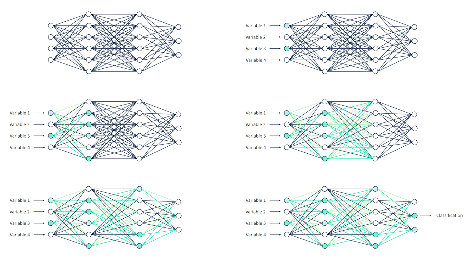
With the weights,inputs and bias term, we multiply the weights with the input and we will add the bias term and then we will perform summation and then we pass this to activation function. This process continues to all the neurons and finally we will get predicted y_hat. This process is called forward propagation.
۳٫ Compute loss function
Difference between the predicted y_hat and the actual y is called loss term. It captures how far our predictions are from the actual target. Our main objective is to minimize the loss function.
۴٫ Back propagation
Here, we compute the gradients and update the weights with respect to loss function . We perform the updation of weights until we get minimum loss.
Steps 2–۴ are repeated for n-iterations till we get minimized loss.
By seeing the above neural network process, we can easily say that, steps 2,3 and 4 functionality is same for any network i.e., we do same operations until we converge to minimum loss, only the big difference for faster convergence to minima in any neural network is right initialization of weights .
Now, let us see the different types of initialization of weights. Before going into the topic ,let me introduce you to some terminologies
Fan-in :
Fan-in is the number of inputs that are entering into the neuron.
Fan-out :
Fan-out is number of outputs that are going from the neuron.
There are two inputs that are entering into the neuron. Hence, fan-in=2.
One output is going away from neuron. Hence, fan-out=1 .
Uniform distribution:
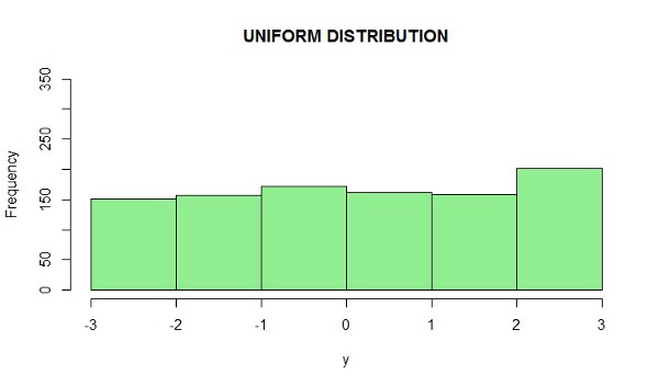
Uniform distribution is a type of probability distribution in which all outcomes are equally likely i.e., each variable has the same probability that it will be outcome.
Normal distribution:
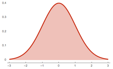
Normal distribution is a probability distribution that is symmetric about the mean, showing that data near the mean are more frequent in occurrence than the data far from the mean.
Now, let us dive deep into the different initialization techniques. From here, we will go in a practical aspect i.e., Let us take MNIST dataset, and we will initialize the weights with different initialization techniques and let us see what’s happening with output.
Overview of MNIST dataset
MNIST dataset is one of the most common datasets used for image classification. This dataset contains hand written number images and we have to classify them into any one of the 10 classes(i.e., 0 – 9).
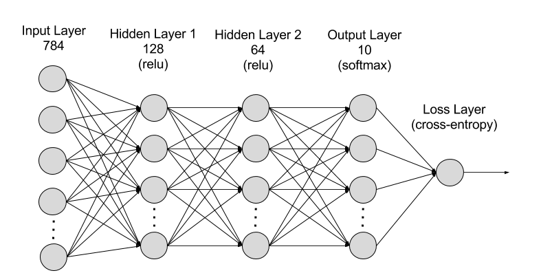
For simplicity, we will consider only a 2 layer neural network i.e., 1st hidden layer with 128 neurons , 2nd hidden layer with 64 neurons and we will a softmax classifier to classify the outputs. Here, we will use ReLU as an activation unit. Ok , Lets get started.
Initializing all weights to zero
Theory
Weights are initialized with zero. Then, all the neurons of all the layers performs same calculation, giving same output. The derivative with respect to loss function is same for every weight. The model won’t learn anything. The weight’s won’t get update at all. Here, we are facing vanishing gradients problem.
Code for initializing all weights to zero
model = Sequential()
model.add(Dense(128, activation='relu', input_shape=(input_dim,), kernel_initializer='zeros'))
model.add(Dense(64, activation='relu', kernel_initializer='zeros'))
model.add(Dense(output_dim, activation='softmax'))
Output for initializing all weights to zero in MNIST dataset.
Epoch 1/5 60000/60000 [==============================] - 3s 55us/step - loss: 2.3016 - acc: 0.1119 - val_loss: 2.3011 - val_acc: 0.1135
Epoch 2/5 60000/60000 [==============================] - 3s 47us/step - loss: 2.3013 - acc: 0.1124 - val_loss: 2.3010 - val_acc: 0.1135
Epoch 3/5 60000/60000 [==============================] - 3s 46us/step - loss: 2.3013 - acc: 0.1124 - val_loss: 2.3010 - val_acc: 0.1135
Epoch 4/5 60000/60000 [==============================] - 3s 47us/step - loss: 2.3013 - acc: 0.1124 - val_loss: 2.3010 - val_acc: 0.1135
Epoch 5/5 60000/60000 [==============================] - 3s 46us/step - loss: 2.3013 - acc: 0.1124 - val_loss: 2.3010 - val_acc: 0.1135
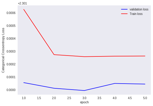
Plot for output values for initializing all weights to zero
Analysis of output
Here, the train loss and test loss are not changing . Hence, we can easily conclude that no change in weights of neuron. From this, we can conclude that, our model is effected with vanishing gradients problem.
Random initialization of weights
Theory
Instead of initializing all the weights to zeros, here we are initializing all the values to random values. Random initialization is better than zero initialization of weights. But, in random initialization we have chance of facing two issues i.e., vanishing gradients and exploding gradients. If the weights are initialized very high, then we will be facing issue of exploding gradients. If the weights are initialized very low, then we will be facing issue of vanishing gradients.
Code for random initialization of weights
model = Sequential()
model.add(Dense(128, activation='relu', input_shape=(input_dim,), kernel_initializer='random_uniform'))
model.add(Dense(64, activation='relu', kernel_initializer='random_uniform'))
model.add(Dense(output_dim, activation='softmax'))
Output for initialization of all weights to random in MNIST dataset
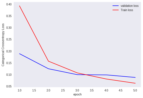
Epoch 1/5 60000/60000 [==============================] - 3s 55us/step - loss: 0.3929 - acc: 0.8887 - val_loss: 0.1889 - val_acc: 0.9432
Epoch 2/5 60000/60000 [==============================] - 3s 45us/step - loss: 0.1570 - acc: 0.9534 - val_loss: 0.1247 - val_acc: 0.9622
Epoch 3/5 60000/60000 [==============================] - 3s 53us/step - loss: 0.1069 - acc: 0.9685 - val_loss: 0.0994 - val_acc: 0.9705
Epoch 4/5 60000/60000 [==============================] - 3s 54us/step - loss: 0.0810 - acc: 0.9761 - val_loss: 0.0986 - val_acc: 0.9710
Epoch 5/5 60000/60000 [==============================] - 3s 54us/step - loss: 0.0629 - acc: 0.9804 - val_loss: 0.0877 - val_acc: 0.9755
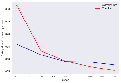
Plot for outputs that their weights are randomly initialized
Analysis of output
Here, the train loss and the test loss are changing much i.e., they are converging to the minimum loss value. Hence, we can clearly say that random initialization is better than zero initialization of weights. But, when we rerun the model, we will be getting different results because of random initialization of weights.
Xavier Glorot initialization of weights
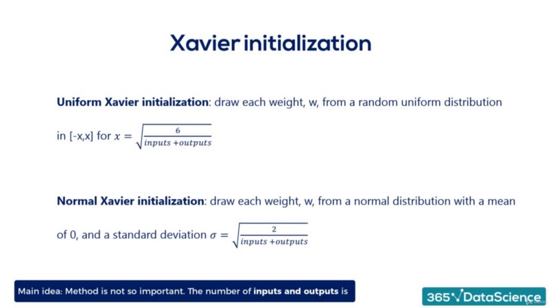
This is an advanced technique in initialization of weights. There are two types of initialization in this i.e., Xavier Glorot normal initialization and Xavier Glorot uniform initialization.
a. Xavier Glorot uniform initialization of weights
Here the weights belong to a uniform distribution with in range of +x and -x, where x=(sqrt(6/(fan-in+fan-out)))
code for Xavier Glorot uniform initialization of weights
model = Sequential()
model.add(Dense(128, activation='relu', input_shape=(input_dim,), kernel_initializer='glorot_uniform'))
model.add(Dense(64, activation='relu', kernel_initializer='glorot_uniform'))
model.add(Dense(output_dim, activation='softmax'))
Output for Xavier Glorot uniform initialization of weights
Epoch 1/5 60000/60000 [==============================] - 4s 68us/step - loss: 0.3317 - acc: 0.9072 - val_loss: 0.1534 - val_acc: 0.9545
Epoch 2/5 60000/60000 [==============================] - 3s 55us/step - loss: 0.1303 - acc: 0.9614 - val_loss: 0.1124 - val_acc: 0.9679
Epoch 3/5 60000/60000 [==============================] - 3s 54us/step - loss: 0.0889 - acc: 0.9731 - val_loss: 0.0978 - val_acc: 0.9711
Epoch 4/5 60000/60000 [==============================] - 3s 54us/step - loss: 0.0668 - acc: 0.9795 - val_loss: 0.0863 - val_acc: 0.9735
Epoch 5/5 60000/60000 [==============================] - 3s 55us/step - loss: 0.0529 - acc: 0.9840 - val_loss: 0.0755 - val_acc: 0.9771
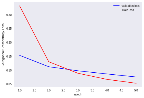
Plot for outputs of Xavier Glorot uniform initialization of weights
Analysis of output
Here, with this Xavier Glorot uniform initialization, our model tends to perform very well. Although ,we can run it multiple times, our output won’t change.
b. Xavier Glorot normal initialization
Here the weights belongs to a normal distribution with mean=0 and variance= sqrt(2/(fan-in+fan-out)).
Code for Xavier Glorot normal initialization of weights
model = Sequential()
model.add(Dense(128, activation='relu', input_shape=(input_dim,), kernel_initializer='glorot_normal'))
model.add(Dense(64, activation='relu', kernel_initializer='glorot_normal'))
model.add(Dense(output_dim, activation='softmax'))
Output for Xavier Glorot normal initialization of weights
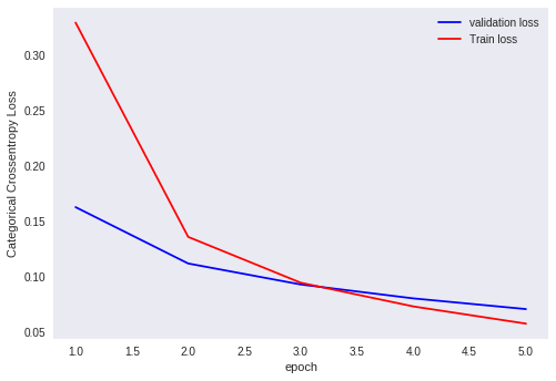
Epoch 1/5 60000/60000 [==============================] - 4s 66us/step - loss: 0.3296 - acc: 0.9064 - val_loss: 0.1628 - val_acc: 0.9492
Epoch 2/5 60000/60000 [==============================] - 3s 50us/step - loss: 0.1359 - acc: 0.9597 - val_loss: 0.1119 - val_acc: 0.9658
Epoch 3/5 60000/60000 [==============================] - 3s 51us/step - loss: 0.0945 - acc: 0.9721 - val_loss: 0.0929 - val_acc: 0.9706
Epoch 4/5 60000/60000 [==============================] - 3s 52us/step - loss: 0.0731 - acc: 0.9776 - val_loss: 0.0804 - val_acc: 0.9741
Epoch 5/5 60000/60000 [==============================] - 3s 51us/step - loss: 0.0576 - acc: 0.9824 - val_loss: 0.0707 - val_acc: 0.9783
Plot for outputs of Xavier Glorot normal initialization of weights
Analysis of output
Here, with this Xavier Glorot normal initialization, our model also tends to perform very well. Although ,we can run it multiple times, our output won’t change .
The weights we set here are neither too big nor two small. Hence, we won’t face the problem of vanishing gradients and exploding gradients. Also, Xavier Glorot initialization helps in faster convergence to minima.
He initialization of weights
It is pronounced as hey initialization . This is also an advanced technique in initialization of weights. ReLU activation unit performs very well with this initialization .We consider only ,number of inputs in He- initialization .In He-initialization also, we have two types i.e., He-normal initialization and He-uniform initialization
a. He- uniform initialization of weights
Here the weights belongs to a uniform distribution within the range of +x and -x, where x=(sqrt(6/fan-in)).
Code for He- uniform initialization of weights
model = Sequential()
model.add(Dense(128, activation='relu', input_shape=(input_dim,), kernel_initializer='he_uniform'))
model.add(Dense(64, activation='relu', kernel_initializer='he_uniform'))
model.add(Dense(output_dim, activation='softmax'))
Output for He-uniform initialization of weights
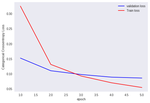
Epoch 1/5 60000/60000 [==============================] - 4s 72us/step - loss: 0.3252 - acc: 0.9050 - val_loss: 0.1524 - val_acc: 0.9546
Epoch 2/5 60000/60000 [==============================] - 3s 52us/step - loss: 0.1314 - acc: 0.9611 - val_loss: 0.1104 - val_acc: 0.9671
Epoch 3/5 60000/60000 [==============================] - 3s 54us/step - loss: 0.0928 - acc: 0.9718 - val_loss: 0.0978 - val_acc: 0.9697
Epoch 4/5 60000/60000 [==============================] - 3s 53us/step - loss: 0.0703 - acc: 0.9786 - val_loss: 0.0890 - val_acc: 0.9740
Epoch 5/5 60000/60000 [==============================] - 3s 53us/step - loss: 0.0546 - acc: 0.9828 - val_loss: 0.0860 - val_acc: 0.9740
Plot for He-uniform initialization of weights
Analysis of output
Here, in He-uniform initialization of weights we are only using the number of inputs. But, only with number of inputs, our model is performing quite descent with the He-uniform initialization of weights.
b. He- normal initialization of weights
Here the weights belongs to a normal distribution with mean=0 and variance= sqrt(2/(fan-in)).
Code for He- normal initialization of weights
model = Sequential()
model.add(Dense(128, activation='relu', input_shape=(input_dim,), kernel_initializer='he_normal'))
model.add(Dense(64, activation='relu', kernel_initializer='he_normal'))
model.add(Dense(output_dim, activation='softmax'))
Output for He-normal initialization of weights
Epoch 1/5 60000/60000 [==============================] - 4s 61us/step - loss: 0.3163 - acc: 0.9087 - val_loss: 0.1596 - val_acc: 0.9508
Epoch 2/5 60000/60000 [==============================] - 3s 45us/step - loss: 0.1319 - acc: 0.9610 - val_loss: 0.1163 - val_acc: 0.9625
Epoch 3/5 60000/60000 [==============================] - 3s 44us/step - loss: 0.0915 - acc: 0.9725 - val_loss: 0.0897 - val_acc: 0.9727
Epoch 4/5 60000/60000 [==============================] - 3s 45us/step - loss: 0.0693 - acc: 0.9795 - val_loss: 0.0878 - val_acc: 0.9735
Epoch 5/5 60000/60000 [==============================] - 3s 44us/step - loss: 0.0537 - acc: 0.9836 - val_loss: 0.0764 - val_acc: 0.9769
Plot for outputs of He-normal initialization of weights
Analysis of output
Here, in He-normal initialization of weights we are only using the number of inputs. But, only with number of inputs, our model is performing well.
In He- initialization also,we set weights neither too big nor two small. Hence, we won’t face the problem of vanishing gradients and exploding gradients. Also, this initialization helps in faster convergence to minima.
How to choose right weight initialization ?
As their is no strong theory for choosing right weight initialization, we just have some rule of thumb methods i.e.,
-
- When we have sigmoid activation function, it is better to use Xavier Glorot initialization of weights.
- When we have ReLU activation function, it is better to use He-initialization of weights.
Mostly, Convolutional neural network will use ReLU activation function and it use’s he-initialization.
Read More :
 شرکت شهاب نرم افزار پلاک خوان | دوربین پلاک خوان | تشخیص چهره


